Natural Language Processing - Deep Learning I

Basic Neural Network Structure

Single neuron, the most basic components of neural networks, consist of multiple inputs $[x_1, x_2, …, x_d]$ and an output $y$. 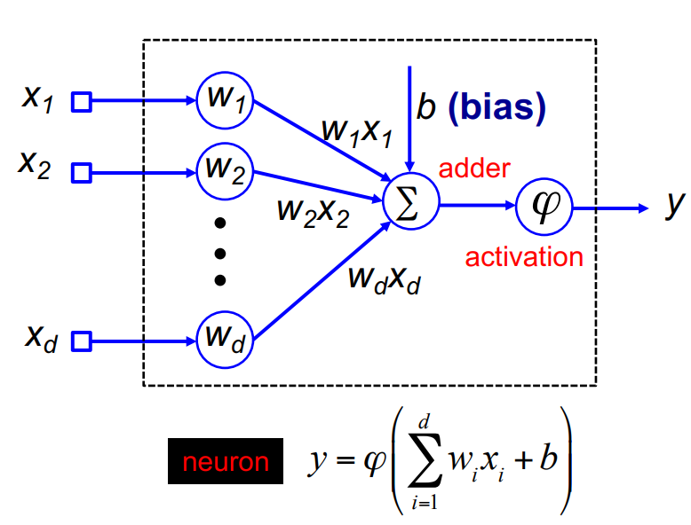The above picture demonstrated, each input $x$ is multiply by a weight $w$, their sum is added with a bias and then activated by a activation function. The training process, is to find the best y value from updating the weight in each training epoch.

Activation function

The meaning of activation function is to give the data non-linear features to allow networks capture more complex changes and pattern. Some common activation functions are: Sigmoid function, Tanh function, Relu function, Parametric Relu and ELU. Each activation function has their own suitable scenario, and we will discuss them in the future.

1. Sigmoid function
   The sigmoid function could returns the data in a range of 0 and 1, the math function and graph is like below: $$ϕ(v) = \frac{1}{1 + \exp(-v)}$$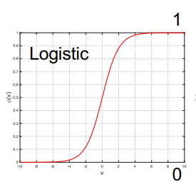

2. Tanh function
   The tanh function could returns the data in a range of -1 and 1. $$ϕ(v) = \tanh(v) = \frac{\exp(2v) - 1}{\exp(2v) + 1} ∈ (-1, +1)$$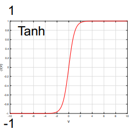

3. Relu function
   The relu function keep the data above 0 normal, and set to 0 to all the data below 0. $$ϕ(v) = \begin{cases} v, & \text{if v ≥ 0} \\ 0, & \text{if v < 0} \end{cases}$$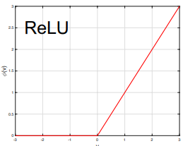

4. Parametric Relu
   The parametric relu function vary the relu function - set data below 0 as $av$, with a = 0.01 in Leaky Relu. $$ϕ(v) = \begin{cases} v & \text{if } v \geq 0 \\ av & \text{if } v < 0 \end{cases}$$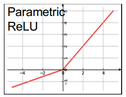

5. ELU
   The ELU function another variants of relu function $$ϕ(v) = \begin{cases} v & \text{if } v \geq 0 \\ a(e^v - 1) & \text{if } v < 0 \end{cases}$$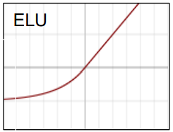

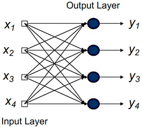
Single Layer Perceptron

A single layer perceptron (SLP) has one input layer and one output layer. Each layer is consist of single neurons.

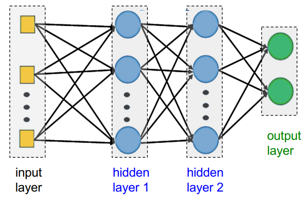
Multilayer Perceptron

A Multilayer Perceptron(MLP), also called a feedforward neural network(FNN), consist of at least a input layer, a hidden layer and an output layer, which each neuron in each layers connected to all neurons in other adjacent layers. The below picture is a feedforward network architecture, here we will introduce it step by step: 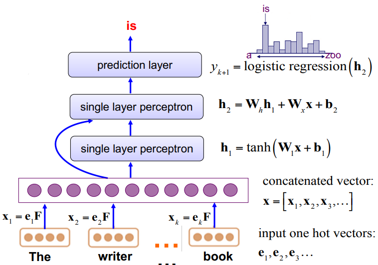Each word input is first processed by an embedding layer, we denote the result of this step as F, after multiply it by one hot vector, we could input it into the network. The concatenated form of all word input is a vector $x = [x_1, x_2, x_3…]$, and we take it to the next formula shown in the picture calculating $h_1$. The next layer uses the output of the previous layer and the product of the weight matrix of the current layer and the input vector(every next layers is calculated like this). And after this we could use a logistic regression function to transform $h_k$ into the predicted output.

RNN

RNN is a type of neural network collecting the last output as the input for next layer, the picture below demonstrate the basic structure of a RNN network. 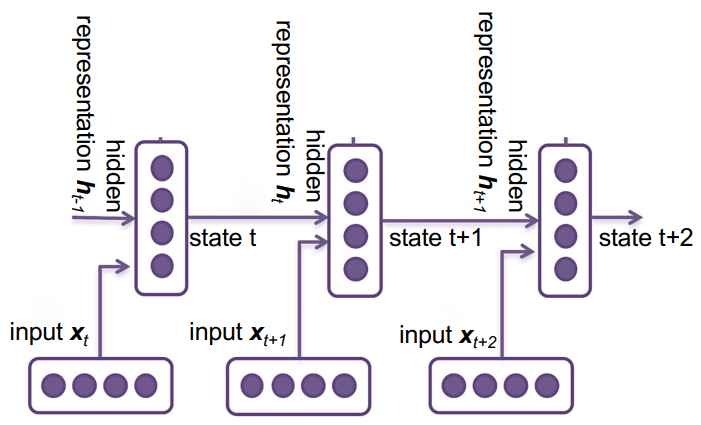As we can see from the picture, the information transmitting in different layers is $h_t$, which consist of three components $x_t$, $h_{t-1}$ and $W$, for example, $h_1 = f(x_1, h_0, W)$(Note that $h_0$ could either be trained or set to a fixed value). $X$ allows multiple means of input, such as output of a feature extractor, word vectors, or directly trained from another neural network. $W$ is the weight, our goal is to get the best weight for generating the best result. The function $f$ could be SLP, MLP that we have already looked at, or we could use LSTM, GRU that we will introduce later. Based on the method we take to calculate $h_t$, there extended some types of RNN: Vanilla RNN, LSTM RNN, GRU RNN…

Vanilla RNN

Vanilla RNN, the most basic RNN, calculating $h_t$ by using a standard neuron operation. The equation is as below: $$h(k) = ϕ(W_xx_k + W_hh_{k−1} + b)$$ The biggest disadvantage of Vanilla is vanishing gradient. What is vanishing gradient? Let’s look at a equation first. $$G_{ki} = (W_{h})^{k-i} \prod_{j=i+1}^{k} D_{j}$$ $W_h$, represents weight in calculating the gradient $G_{ki}$, might be vanishing or explosion with respect to $k-i$, where k is the state of interest and i is the previous state. This leads to a short-term memory of the model or unstable ’learning’ process and inefficient. In this case, we could make some changes to to the standard neuron operation, and we have LSTM RNN and GRU RNN.

LSTM RNN

The idea of LSTM RNN is to add multiple gates to control input of current and previous content vector and output. First of all, copy the operation of standard neuron operation, change the activation function to tanh, and name the new operation as $c_k$ to represents the updated information about current state. $$c_k = tanh(W_xx_k + W_hh_{k−1} + b)$$

Afterwards, we could define the equation of $h_k$ (The · symbol represents element wise multiplication). $$h_k = o_k · tanh(f_k · c_{k-1} + i_k · c_k)$$

There are three gates in the equation, which $o_k$ represents the output gate, $f_k$ represents the forgot gate, and $i_k$ represents the input gate.

1. Output Gate
   The output gate controls the selection of which numbers could be return in the mixed of both previous and current content vectors. The equation for $o_k$ is: $$o_k = σ(W^o_xx_k + W^o_hh_{k-1} + b^o)$$
2. Forgot Gate
   The forgot gate controls which numbers in the previous state are selected. The equation is: $$f_k = σ(W^f_xx_k + W^f_hh_{k-1} + b^f)$$
3. Input Gate
   The input gate controls which numbers in the current state are selected. The equation is: $$i_k = σ(W^i_xx_k + W^i_hh_{k-1} + b^i)$$

By the control of gates, the LSTM function could have a kind of long-term memory.

GRU RNN

Due to the fact that LSTM RNN has too many parameters, therefore it has a slow running speed. Therefore, compare to LSTM RNN, GRU RNN keeps the idea of gates, but it decreases the gates and parameters it used to optimize the running speed. An equation for calculating content vector $c_k$ is shown below: $$c_k = tanh(W_xx_k + W_h(r_k·h_{k−1}) + b)$$ Within the equation for $c_k$, we have a reset gate which having similar function as forgot gate, it selects which numbers in the previous representation vector to use. The equation for it is as below: $$r_k = σ(W^r_xx_k + W^r_hh_{k-1} + b^r)$$ And the equation for $h_k$ is: $$h_k = (1-u_k) · h_{k-1} + u_k · c_k$$ $u_k$ represents the update gate. It selects for both previous representation vector and current content vector about which numbers to use. The equation for update gate is: $$u_k = σ(W^u_xx_k + W^u_hh_{k-1} + b^u)$$

RNN Application: Seq2seq Model

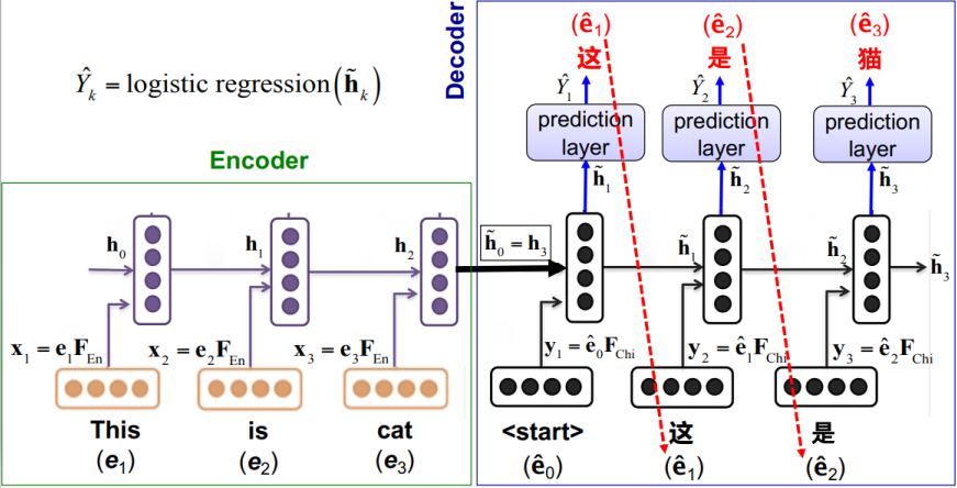The above picture is an example of a seq2seq model, we could see that it contains two separate parts: encoder and decoder. They have different responsibilities in this model. First of all, the encoder works as normal RNN, recursively process each input word vectors and calculating each $h_k$ by using vanilla or LSTM or GRU RNN. Then for the last representation vector of encoder $h_3$, make it as the first representation of decoder $\tilde{h}_0$, combining it with <start> as the first content vector. After a list of calculation, we got $\tilde{h}_1$, now we could use a logistic regression function $\tilde{Y}_k$ to transmit our vector into a Chinese word, where in the example, “这”. This Chinese word will be used as the next input word vector, and keep running until the ends.

Advanced RNN Architectures

Except LSTM and GRU RNN, we still have another two advanced RNN architectures, with their structure changed instead of calculations. They are bi-directional RNN and multi-layer RNN.

Bi-directional RNN

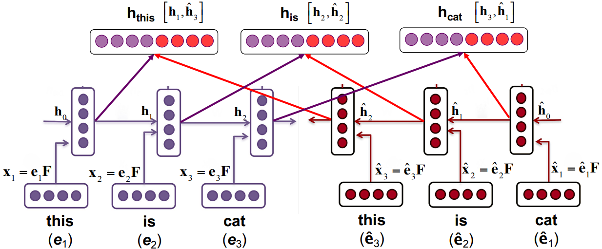
The motivation for bi-directional RNN is to take care of both left and right context, as the representation vectors could be influence by both left and right representation vectors. In this case, we use two RNNs with original and reversed input respectively. The picture below demonstrate a structure of bi-directional RNN:

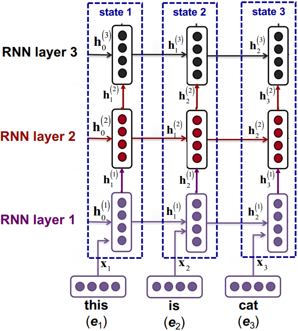
Multi-layer RNN

The motivation for multi-layer RNN is to compute more complex representation vectors and improve model performance. To achieve this, we could stack multiple layers of RNN, normally 2 - 4 layers.

---

• ← Previous Post
• Next Post →