In this article we will have a look at how to represent texts in data forms for further nlp processes.
BoW Representation
BoW - “Bag of words”, should be the simplest model, which reduce each document into a bag of words.
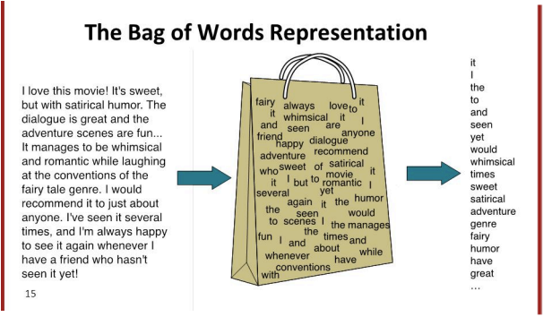
BoW is an efficient method which nowadays lots of NLP system is using it. However, there are some question we should think of while using it, such as:
- Are all the words equally important?
- What about (important) combinations of words?
- What about negations?
- Is the meaning lost without order?
In this case, we should find some methods to solve all these problems. Let’s look at some theories first.
Zipf’s Law
All words in our text has frequency, some words are very frequent, such as “the”, “a”, “as”, etc. And some other words is not very frequent, like “bazinga”. There are about 50% terms appears once only, therefore we have Zipf's Law announced by George Zipf, which states that: frequency of any word in a given collection is inversely proportional to its rank in the frequency table.
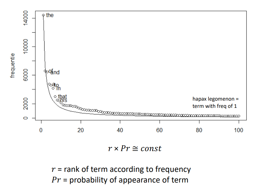
Luhn’s hypothesis, is a theory based on Zipf's Law, defining upper cut-off and lower cut-off, states that the range of words between these two cut-offs are the words help figuring the exact meaning of texts.
Removing Stop words
Based on the Zipf’s law, we could define stop words, which are the highly occurring words with less distinguishing power for representing documents. In this case, we could filter them for a cleaner data and faster process speed. However, not all nlp application will benefit from removing stop words, and for different purposes, we should use different list of stop words.
Vector Representation
The vector representation is a way of implementing the BoW model. We have two method of defining the vector representation. The first one is by incident(0 or 1), which define a vocabulary V consist all words left after all pre-processing procedures, and each document is represented by a V dimensional vector with occurred words in 1 and others in 0.
$$ d = [w_1, w_2, … , w_{|v|} ] $$
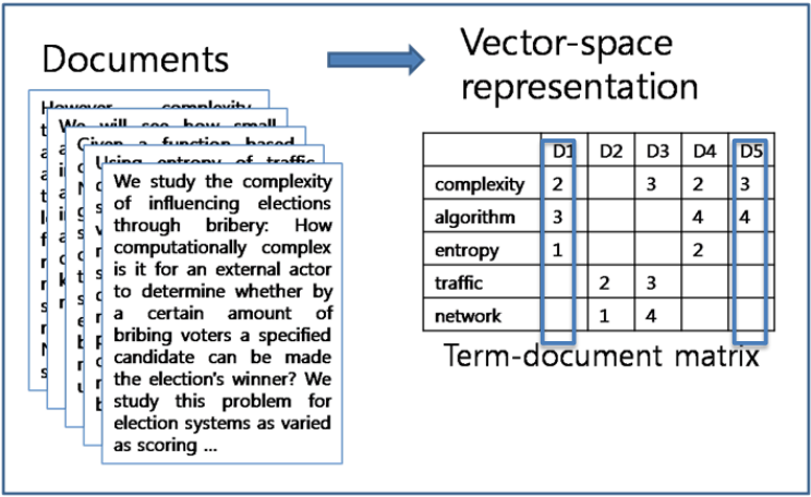
The second method is by matrix, which is shown in the following picture.
Weight
In order to let our representation more accurate, it is better to consider weight. The most easiest way is counting the occurrence number of each words. However, consider Zipf’s law again, the words occurs many times doesn’t mean it is more important. Thus, we have tf.idf weighting.
TF.IDF Weighting
Before we introduce tf.idf, we should know what is document frequency and inverse document frequency. Document frequency is the number of documents that contains term t, in other words, It is a measure of “informativeness” of t. And we could calculate the idf(inverse document frequency) by using the following equation.
$$ idf_t = log_{10} (N/df_t) $$
In the equation, N is the total number of documents. If the result is high, then it means the term appears in few documents, and vise versa.
The tf.idf weighting is calculated by multiplying term frequency weight and inverse document frequency weight, the equation is as below:
$$tf.idf_{t, d} = (1+ log_{10}tf_{t,d} )× log_{10} (N/df_t)$$
It will increase with the number of occurrences within a document and the rarity of the term. By replacing the weight in a matrix vector representation, we got a more accurate result.
Language Models
From now on let’s have a look at some language models.
N-gram Language Models
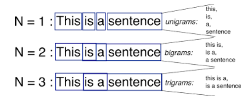
Think about a situation when we dealing with words like “The United States”, building representation with each word separately doesn’t show the correct meaning, in this case, we could build a n-gram model to solve this kind of problem. Below is a picture showing the effects of different n number.
Probabilistic Language Models
Consider a sentence, “I saw a rabbit _______ yesterday”, what do you think is a better word to fill in the blank? It is true that “running” is more likely to be here rather than “flying”. By following this idea, we could use probabilistic language model to measures the probability of natural language utterances, giving higher scores to those that are more common, more grammatical, more “natural”.
Unigram Language Models
The first method we could use to add probabilistic in model is unigram language models. In any sequences of words $S = w_1, w_2, …, w_n$, the probability could be calculate as (assume all words appeared independently and identically distributed, although it is wrong, but it words well in some nlp applications):
$$p(S) = p(w_1) * p(w_2) * … * p(w_n) = \prod_{i} p(w_{i})$$
Now, the question is, how to we know all the probabilistic? Here we could use corpus frequencies - count how many times the words appear in a real-world dataset, and normalize by using the total number of words in the corpus, below is the equation:
$$ p(w) = \frac{|w|}{\sum_{t} |t|} $$
Additionally, we have to consider OOV(Out of Vocabulary) words, we can’t just let $p(OOV) = 0$ because thus we can never use our model on unseen words. Therefore we could add a add-one smoothing, the changed equation is as below:
$$ P(w) = \frac{|w| + 1}{\sum_{w’ \in D} (|w’| + 1)} $$
However, there’s still a disadvantage of the current language model we use(not only unigram, but also bigram, trigram…) - it completely loss order information, and the following situation might exist:
$$p(\text{“the the the the ”}) > p(\text{“the cat in the hat ”})$$
It is completely unreasonable! In this case, we could apply chain rule.
Chain Rule
By using chain rule, the probability could be calculated as below:
$$p(w_1, w_2, w_3, …, w_L) = p(w_1) p(w_2 | w_1) p(w_3 | w_1, w_2) … p(w_L | w_1, w_2, \ldots, w_{L-1})$$
Or, in a simple form:
$$\prod_{k=1}^{L} p(w_k | w_1, w_2, \ldots, w_{k-1})$$
Markov Assumption
The question now is, it is quite complicated to calculate by using all previous probabilities. Thus, Markov assumption could be implemented to simplify this case, as we only need to consider the previous words into account. An example could be $p(hat\ |\ the\ cat\ in\ the) ≈ p(hat\ |\ the) $. Afterwards, the equation for unigram language model is:
$$p(w_{1:L}) = \prod_{k=1}^{L} p(w_k\ |\ w_{k-N+1:k-1}) = \prod_{k=1}^{L} p(w_k)$$
N represents the n of n-gram model, we only care about N-1 previous words, so for unigram we still use the probability of single words, but the equation of bigram model is:
$$p(w_{1:L}) = \prod_{k=1}^{L} p(w_k\ |\ w_{k-N+1:k-1}) = \prod_{k=1}^{L} p(w_k\ |\ w_{k-1})$$
Count-based Estimation
Before we mentioned the corpus frequencies could be use to calculate the single-word probabilities, but how do we calculate when more than one word is being processed? Here we have count-based estimation.
$$p(w_k\ |\ w_{k−1}) = \frac{count (w_{k−1}w_k)}{\sum_{w}{count(w_{k-1}w)}} = \frac{count (w_{k−1}w_k)}{count(w_{k-1})} = \frac{C(w_{k-1:k})}{C(w_{k-1})}$$
The $count (w_{k−1}w_k)$ means the total number of the combination of word $w_{k-1}$ and $w_k$ appearing together, and we normalize it by dividing the total number of $w_{k-1}$ and any other words appearing together. To generalize it to n-gram, we change it to the following equation: $$\frac{C(w_{k-N+1:k})}{C(w_{k-N+1:k-1})}$$
An Example
Combining all the knowledge above, let’s have a look at an example:
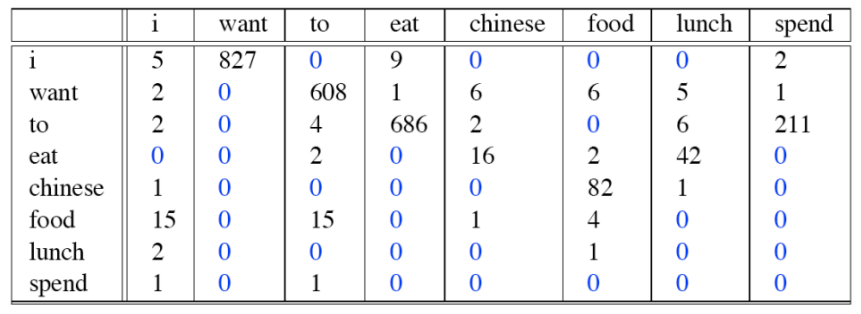
 The first graph demonstrate the counts of each bigram appearances, and the second one is the total number of each words in the corpus. If we want to know $p(to\ spend)$, we could first read the count of “to spend” in the table, which is 211, then divided by 2417, the occurrence number of “to”, and the result is 0.087.